Compiling Neural Networks for a Computational Memory Accelerator

I will be presenting a short paper entitled Compiling Neural Networks for a Computational Memory Accelerator in the SPMA workshop. This is was my main project over my last year at IBM research. The goal of the project was to build a software system stack for a computational memory accelerator developed in our lab. The paper presents some early progress towards this goal. Since I left IBM on February, this project has been more or less on a hiatus. With the presentation coming up, I wanted to write some notes for my own benefit but also try to engage the community and see what other people think about this.

The TL;DR version is: accelerating inference with analog computational memory accelerators based on technologies like PCM or Flash is promising but it depends on using pipeline parallelism. To use pipeline parallelism we need a way to enforce data dependencies between cores. There is a neat way we can do that using polyhedral compilation.

Computational Memory

Computational memory (CM), sometimes also referred to as in-memory computing, realized with analog hardware is a rich area of research. The first obvious question is whether it offers a benefit compared to traditional digital design. There are people that do not think so, and people that do. Here, I will assume that it does offer a benefit, and will also narrow it down to a specific hardware unit: an analog unit that can perform a Matrix-Vector multiplication (MxV) operation. These units are typically implemented as crossbars arrays, so I will be using that term as well.

In contrast with traditional digital designs where memory and computation happens in different units, our analog MxV unit does both. It holds the data of the matrix, and also performs the MxV operation when we feed an input vector into it. The MxV operation happens in two steps. First we program the crossbar with the matrix (M). Subsequently, we can provide a vector (V) as input and get the result (MxV) as output. (An apt analogy from the software world would be partial evaluation.)

Accelerating inference on Neural Networks

In our work, we do not want to use CM for general-purpose computing. Instead, our goal is to use it to accelerate neural network (NN) inference. This is important because some of the tradeoffs of analog computing (e.g., lower precision) are acceptable in this domain. It might be worth mentioning that NN accelerators are quite a hot topic these days.

From a computational perspective, a neural network is a dataflow graph of operators. Operators have weights which are computed during the training phase, and are read during the inference phase. The broad idea of our approach is accelerate inference by storing the weights in the CM units.

For example, we can execute the convolution operator using the MxV hardware unit. (For the curious, here’s some python code on how convolution can be implemented with MxV.) The convolution operator is important enough to have a popular class of NNs named after it, and, unsurprisingly, most of the execution time in these networks is spent on convolutions.

Now might be a good time to have a look at digital accelerators, and how they work. While there are many of them out there, a great example is NVIDIA’s NVDLA. This is an open architecture with comprehensive documentation and a open source software stack to go with it. An NVDLA core has a number of different hardware units for the most common NN operators, including a convolution core.

NVDLA works by executing one layer at a time¹, as do most accelerators. For a CM accelerator, this would mean that for every layer: we program the crossbar with the appropriate weights, we execute a batch of operations, and then we reprogram the crossbar for the next layer. Unfortunately, some of the technologies like PCM or Flash used to build crossbars take such a long time to program that this is not a viable option. Hence, for these accelerators to work well in practice, all (or at least most) of the dataflow program that is the NN has to fit into the accelerator. In this case, the crossbars can be programmed once for each different network and then inference can be performed by streaming data through the accelerator and receiving the output. In my opinion, this characteristic, i.e., that it is too expensive to change weights, is what differentiates CM accelerators both in terms of hardware architecture and system software design from existing accelerators.

One question that the above raises is what happens if there are insufficient hardware resources for a particular network to fit on an accelerator. In that case we might try to compress the network, potentially loosing an acceptable amount of accuracy, or we might even develop specific training methods that aim to achieve maximum accuracy while producing a network that can be executed on a given accelerator. For the time being, I will assume that the accelerator has ample resources to fit a given network.

The simplest example

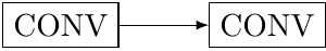
Having said that, let’s try out a simple example to make things more specific. Let’s say that we have the following dataflow graph to execute on our accelerator: a convolution that feeds into another convolution.

To keep things simple let’s also assume that these convolutions are one-dimensional. Specifically, our image is an one-dimensional array of size 10 and for each convolution has single filter of size 3. Let’s start by write down the code for a single such convolution in python.

import numpy as np

# simple one-dimensional convolution kernel
def conv_simple(inp, filt, out):
    (out_size,) = out.shape
    (filt_size,) = filt.shape
    for w in range(out_size):
        outw = 0
        for k in range(filt_size):
            outw += inp[w + k] * filt[k]
        out[w] = outw

W1 = 10 # image size
K = 3   # filter size

i = np.random.rand(W1) # input
f = np.random.rand(K)  # filter
W2 = (W1 - K) + 1      # result size
r = np.zeros(W2)       # result array

conv_simple(i, f, r)

The fist thing we want to do for using our CM accelerator is to transform our convolutions to use the MxV operation. One way to do this is shown below. Note that this a degenerate case because the output vector of the MxV operation consists of a single element, while it would normally consist of multiple elements (one per filter). We verify that the result is the same in both cases, so hopefully all is good.

def conv_simple_mxv(inp, filt, out):
    (out_size,) = out.shape
    (filt_size,) = filt.shape
    for w in range(out_size):
        v = inp[w:w+filt_size]
        out[w] = np.matmul(v,filt)

r1 = np.zeros(W2)
conv_simple_mxv(i, f, r1)
np.testing.assert_allclose(r1, r)

Actually, we can write the code differently to better illustrate how our accelerator would work by including the phase where we program (configure) the crossbar, as shown below. In python, “configuration” is just wrapping a function with a given argument, but in an actual CM core this is when we would configure the crossbar with specific weights.

class Crossbar:
    def __init__(self):
        self.mxv = None
        self.K = None

    def configure(self, m):
        (self.K,) = m.shape
        self.mxv = lambda v: np.matmul(v, m)

    def conv(self, inp, out):
        (out_size,) = out.shape
        for w in range(out_size):
            v = inp[w:w+self.K]
            out[w] = self.mxv(v)

r2 = np.zeros(W2)
xbar = Crossbar()
xbar.configure(f)
xbar.conv(i, r2)
np.testing.assert_allclose(r2, r)

Now, let’s go back to our two convolution graph (CONV1 -> CONV2) and try to execute this on a CM accelerator that has two cores, each with its own crossbar.

One option would be to use data parallelism, where we split each convolution computation to multiple cores. In our simple example, where the output of the first convolution is just 8 elements, the first core can compute r[0..4] and the second r[4..8]. Once both cores are finished we can do the same for the second convolution. The problem with this approach, as we mentioned earlier, is that we would have to reprogram the weights (filters) on the crossbars for the second convolution, which would take a significant amount of time and result in poor performance.

A better option would be execute the code on the two cores of our accelerator using pipeline parallelism by executing each convolution on a different core. This is depicted in the figure below. The first convolution is executed on Core 1 reading from array a and writing to array b, while the second convolution on Core 2 reading from array b and writing to array c which is the final result. (Note that we can combine both parellizing strategies. If our accelerator had 4 cores, for example, we could build two different pipelines, each running in parallel computing a different region of the output.)

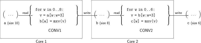
As shown in the figure, each core has some local memory to store input data of the code it executes, and there is also an interconnect that allows Core 1 to write to the local memory of Core 2.

So far so good: we have assigned the two convolutions of our (very simple) dataflow graph to the two CM cores of our accelerator. The next question, is how we control the execution of these two operations since they are dependent: the input of CONV2 is the output of CONV1. One solution would be to wait until CONV1 has finished and b is fully written. This, however, negates pipeline parallelism because the two convolutions would run sequentially. Looking at this example, after 3rd iteration of CONV1, the dependencies for the 1st iteration of CONV2 (b[0:3]) are available and it may start without having to wait for all of b to be written.

It seems like to compile NNs for our CM accelerator, we need some control logic that enforces data dependencies between computations running on different cores. Can we somehow generate this logic in a manner that can work for arbitrary NNs? To do so, we need a framework that allow us to express code dependencies of different loops in a formal manner. Enter polyhedral compilation.

Polyhedral compilation

We will use the polyhedral model, which was originally developed for automatically parallelizing code but has since been used in many different applications. In the polyhedral model, computations are represented as nested loops that access multi-dimensional arrays. Since most nodes on NN dataflows are linear algebra operators with tensor operands, the polyhedral model works well for NNs.

Specifically, we will be using the ISL library, which implements an efficient representation of sets of integer tuples and maps that map elements of one ISL set to another. Specifically, ISL sets are used to model iteration spaces, where each tuple consists of the values of the induction variables of a loop nest, as well as array locations, where each tuple is a multi-dimensional index into the array elements. ISL maps (also called relations) are used to expressed mappings between such sets (e.g., data dependencies). If you want to learn about polyhedral compilation using ISL, check out Presburger Formulas and Polyhedral Compilation.

Let’s have a look at our example to make things concrete. Because CONV1 is a single loop nest, its iteration space is defined by tuples with a single element: \((w): (0), (1), \ldots, (7)\). (In the general case, there would be multiple loop nests and so the tuples would have multiple dimensions.) We can express the CONV1 iteration space in ISL as follows:²

import islpy as isl # ISL python wrapper: https://pypi.org/project/islpy/
isl.Set("{ CONV1[w] : 0 <= w < 8 }")

We can also represent the elements of a multi-dimensional array as an ISL set where each integer tuple represents the dimensions of an element. For array a (again, a in our example is one dimensional, but this is not true for the general case):

isl.Set("{ a[i] : 0 <= i < 10 }")

Furthermore, we can also use ISL to express the accesses that our code performs. For example, CONV1 accesses two arrays: it reads from a and writes to b. We use ISL maps to express how each iteration access these arrays. An ISL map maps elements from a set to elements of another For reads, the access relation maps elements from the iteration space (CONV1[w]) to elements of a (a[i]). Similarly for writes, and for CONV2. Specifically, we can express these relations in ISL as follows:

conv1_rd = isl.Map("{ CONV1[w1] -> a[i1] : 0 <= w1 < 8 and w1 <= i1 < w1 + 3 }")
conv1_wr = isl.Map("{ CONV1[w1] -> b[j1] : 0 <= w1 < 8 and j1 = w1 }")
conv2_rd = isl.Map("{ CONV2[w2] -> b[j2] : 0 <= w2 < 6 and w2 <= j2 < w2 + 3 }")
conv2_wr = isl.Map("{ CONV2[w2] -> c[k2] : 0 <= w2 < 6 and k2 = w2 }")

For example, iteration w=3 of CONV1 will read a[3], a[4], and a[5] and write to b[3]. These relations can be extracted from code (this is how compilers using polyhedral compilation work), but also, in our case, specified for each operator in a NN.

The ISL library provides a set of operations for manipulating these relations. Using these operations, we can build a relation \(\mathcal{S}\) such that it maps observed writes in b, to the maximum (based on execution order) iteration in CONV2 that can be executed. This allows to implement the control logic that we need to enforce data dependencies between the two cores.

I will not dive into the details of how this relation is computed in this post, but you have a look at the appendix of our paper and also our prototype code if you are interested.

For our specific example, the relation would like this:

  >>> isl_rel_loc_to_max_iter(conv1_wr, conv2_rd)
  Map("{ b[j1] -> CONV2[w2 = -2 + j1] : 2 <= j1 <= 7 }")

So, using this relation we can deduce that once we observe a write at b[4] we can execute all iterations up to and including w=2 on CONV2.

In our prototype we use this relation and ISL's code generation facilities to generate a state machine that snoops writes from other cores and controls the computation of the local core so that data dependencies are respected.

Conclusion

The benefit of using polyhedral compilation is that if you can express the accesses using ISL, then you don’t really care if this is a convolution or any other operation. The control logic will just work. Moreover, you can apply optimizations in code (e.g., by changing the order of computations) and the control logic will still work. So I do think that our approach shows promise. With that being said, however, this work is still in the early stages.

As I’ve hinted a couple of times already, we ‘ve published the code that realizes these ideas on github which includes some more complex examples that the one I described here.

Footnotes